MEASURING THE E-FIELD PRODUCED BY AN MRI MACHINE

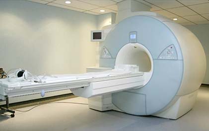
The Kapteos eoSense Converter and eoProbe solution allows you to measure the exposure of people to electromagnetic fields generated from an MRI. The radio frequencies field analysis requires a very high spatial resolution that the Kapteos solution can provide.
The measurements can be performed under a magnetic field of 3 or 4.7 Tesla, depending on the MRI model.

Example of specific projects:
 Measurement tests of electric fields under 3 and 4.7 Tesla
 Vectorial E-field mapping inside a phantom exposed to 100 MHz EM waves generated by an hyperthermia applicator inside a MRI machine

 Application Note: Measuring the E-Fields produced by an MRI Machine

Application Note:

Pulsed EM field with high frequency carrier: How to measure weak RMS signals using a Spectrum Analyzer in time domain

Background

This application note explains how to perform measurements of pulsed electric fields using an Automatic Spectrum Analyzer (ASA).

This technique applies in two particular cases:

• When the oscilloscope does not cover the useful frequency bandwidth

• When the signal delivered by the eoSense Converter is too low to be acquired with an oscilloscope due to noise integration over the whole bandwidth.

The technique presented here is the measurement of a signal from a MRI machine, but may be used in any other applications presenting the same need of measuring a low magnitude electric field using a spectrum analyzer in time domain. The other applications may be repetitive EMPs, radars, etc.

Experimental setup and ASA parameters

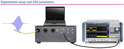
The above picture shows the following elements from left to right:
• The signal to be measured
• The electro-optic probe (eoProbe) connected to the channel 1 input of eoSense optoelectronic converter
• The eoSense converter (with its laptop) output channel 1 connected via a coaxial cable to an Automatic Spectrum Analyzer (ASA)
• An Automatic Spectrum Analyzer (ASA)

The eoSense delivers an analogue signal which is an image of the field vector component to be measured. This analog signal is generated in real time and includes magnitude and phase information over the whole bandwidth of the eoSense optoelectronic converter.

Key Point:
Parameters to extract and record useful information using an ASA:
• The central frequency ƒ0 [Hz]: it has to be fixed to the carrier frequency ƒc
• The span SP [Hz]: it should be tuned to zero (“zero span” mode also called “time mode”)
• The resolution bandwidth RBW [Hz]: its value is crucial; it should be as low as possible to keep a low noise floor while being large enough to contain the spectral (Δƒ) useful information of the signal
• The sweep time ST [s]: it should be in line with the pulse duration (t) and repetition rate of the pulses (ƒREP)
• The trigger level [dBm] or [V]: it has to be adjusted to a fixed value allowing the visualization of the whole pulse (video trigger). Non applicable in case of an external trigger

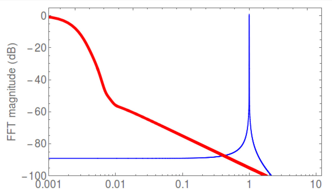
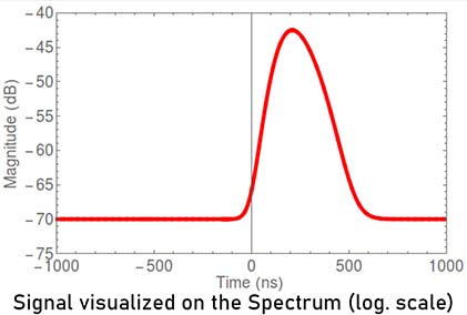
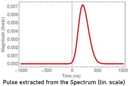
The pulse (red curve) is here asymmetric with a duration of 600 ns. The carrier frequency (blue curve) is ƒ0 = 1 GHz (period of 1 ns). The temporal evolution of the signal is given above with the associated spectra. A typical measurement using an ASA in frequency domain would lead to the blue curve of the Spectrum. The zero span mode could be used to extract shape and magnitude of the pulse envelope using the following parameters:

• Span SP = 0Hz (time domain)
• Carrier frequency ƒ0 = 1 GHz
• RBW = 10 MHz. RBW >~ Δƒ ~ 2 MHz (maximum to cover the spectrum bandwidth of the envelop down to -60 dB)
• Sweep time ST = 2 μs >~ 0.6 μs (to get the whole pulse)

The extracted pulse is usually expressed in Volt and has to be multiplied by the antenna factor to retrieve the temporal evolution of the RMS (root mean square) electric field.

 Keep in mind:
• ƒ0 = ƒc
• SP = 0
• RBW >~ Δƒ
• Δt ~< ST < 1/FREP

Application Note: How to measure weak RMS signals using a Spectrum Analyzer in time domain