
KAPTEOS PRODUCT LINE
The Value and Benefits of Electro-optic Technology
Kapteos Products
• eoSense™ Optic to Electro Converter
• eoProbe™ to measure E-field (EMF)
•• eoCal™ – eoProbe Calibration
•• eoLink™ – 100m Fiber optic extension
•• eoPod™ – eoProbe Articulated Arm and Stand
Kapteos – On-Site Training
• Applications (Target Markets)
• Antennas – Measurement of E-fields Emitted by Antennas• NFACS (Near Field Antenna Characterization Solution)
• 3D NFACS (Near Field Antenna Characterization Solution)
• Vectorial & Characterization of Ultra Compact Antennas
• EMC -Measurement of E-Fields in Electromagnetic Compatibility
• EMP – Time-resolved measurements of Electromagnetic Pulse
• High Temperature – Measurement in High Temperature
• High Voltage – Measurement of E-fields in High Voltage
• Measuring the E-Field around a Laptop
• MRI – Measurement of E-fields inside an MRI
• Plasma – Measurement of E-fields inside Plasma
• SAR – Specific Absorption Rate (SAR) assessment
• Online Software Simulation Tool – Determine Online, before you purchase, the value of the Kapteos Solution!
• FAQ’s – A wealth of Information!
RELIANT EMC PRODUCT LINES
MANUFACTURERS
Request a Quote / Contact Us!
KAPTEOS CHARACTERIZATION OF COMPACT ANTENNAS
VECTORIAL E-FIELD MEASUREMENT & CHARACTERIZATION OF ULTRA COMPACT ANTENNAS
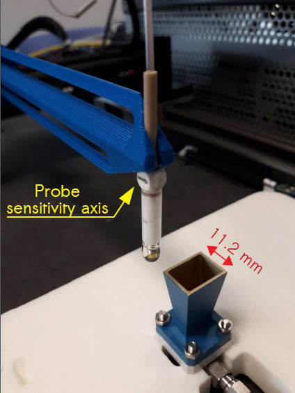
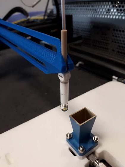
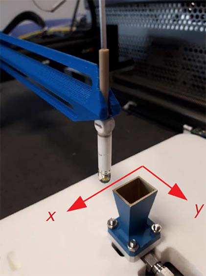
Typical experimental setup
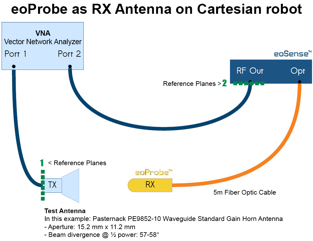
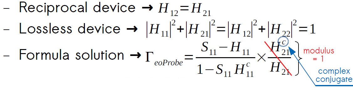
DIFFERENCE BETWEEN OPTICAL & RF RX LINK
– NO SIMPLIFICATION FOR RF RX LINK
– FOR OPTICAL RF LINK:
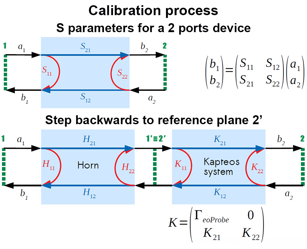
Perfect isolation S12 =
Output RL (Return Loss) given only by eoSense R
Input RL linked at 1st order only to horn R
Chain IL simply equal at 1st order to ILhorn x ILeoSystem
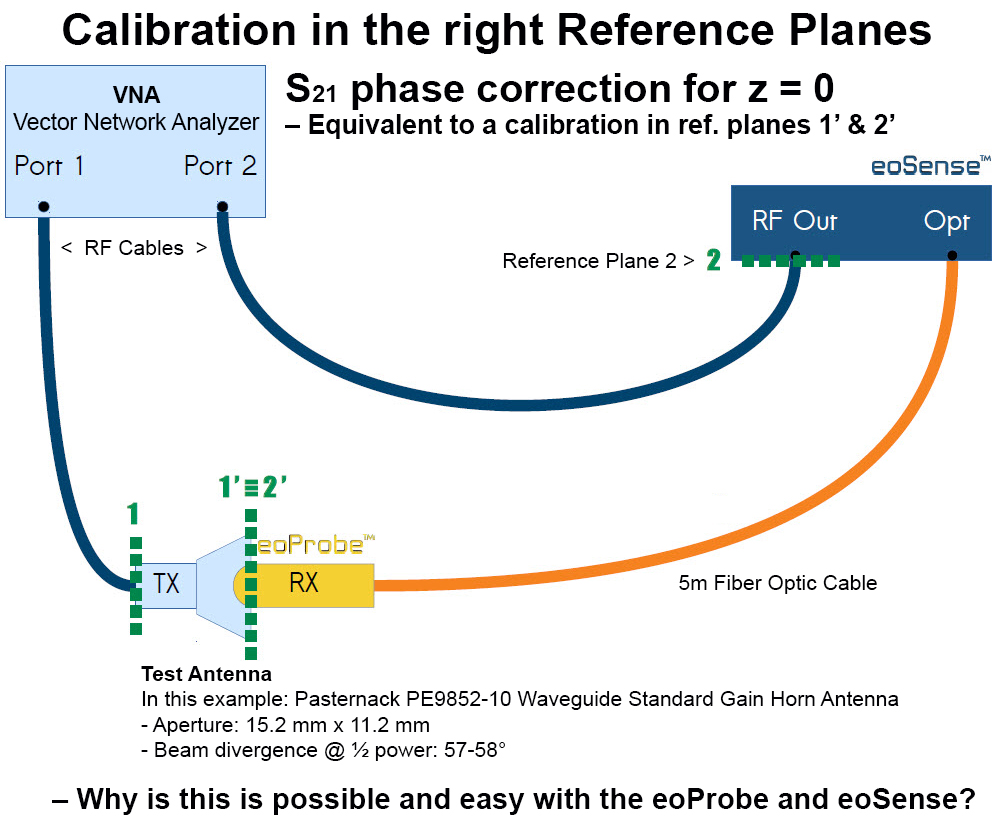
THE ADVANTAGES OF THE KAPTEOS OPTICAL RX LINKS ARE:
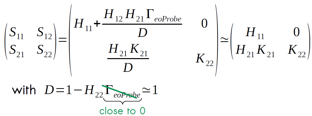
– Rigorously perfect isolation K12 = 0
– Almost infinite input Return Loss K11 ≃ 0
– Whatever DUT upstream Kapteos system rigorously perfect decoupling of output Return Loss S22 = K22
– Straightforward de-embedding of Kapteos system
Insertion Loss ← H21 ≃ 0 S21 / K21
For magnitude → Scalar Kapteos system calibration Scalar Kapteos system calibration
For phase → Scalar Kapteos system calibration Straightforward post-treatment
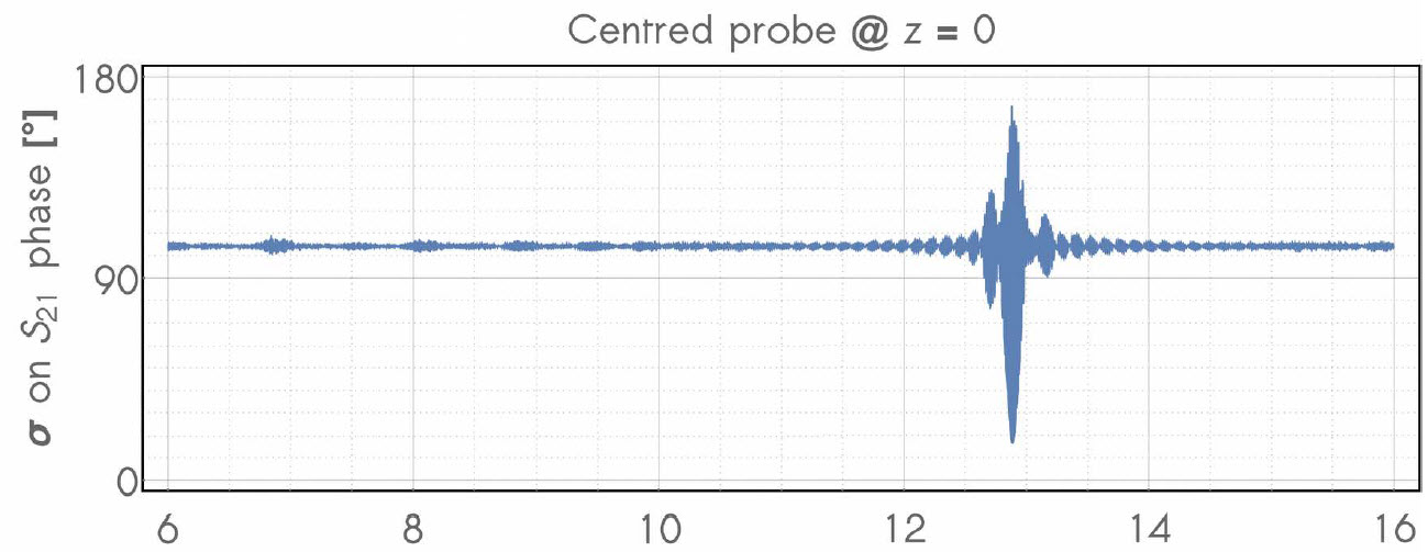
- K21 SUBSTRACTION
– Minimum on σ on φS21 for βL/f = 12.89 °.μs
- – Phase accuracy → 1.7°
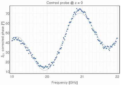
USE OF MEASUREMENTS
- Evolution of corrected phase with z
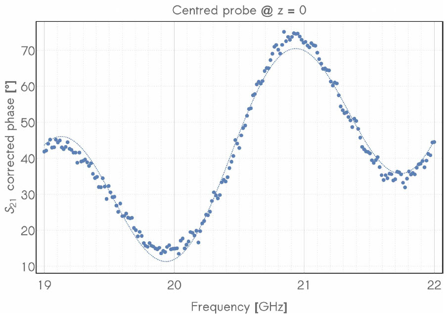
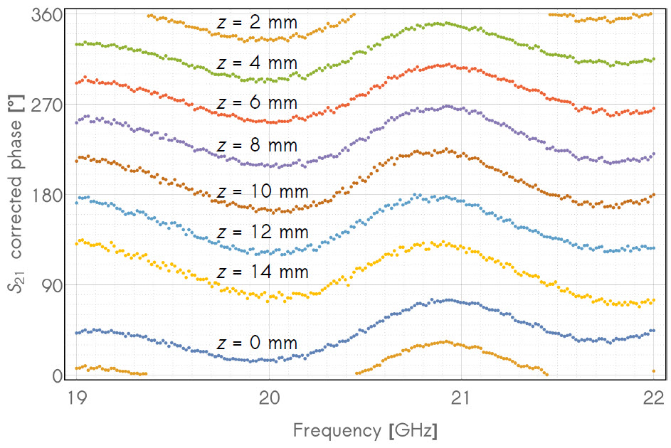
Evolution of S21 corrected phase with z
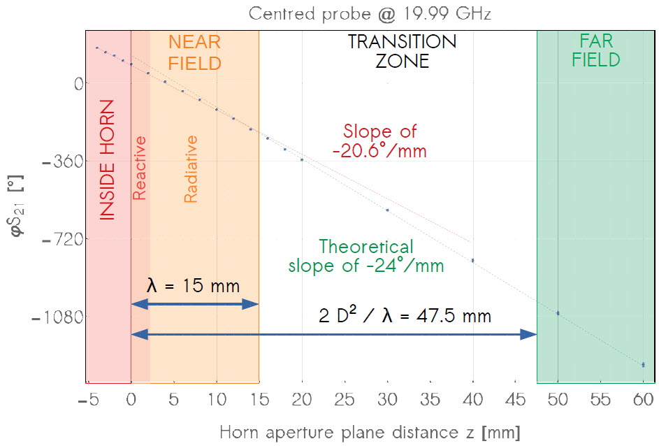
EVOLUTION OF S21 CORRECTED PHASE WITH Z
– Perfect agreement with theory
- In far-field region
- In transition zone
– Lower phase slope in near field region
- Due to effective permittivity ≠ 1 in presence of optical probe
- Phase velocity can be deduced
– Effective optical probe permittivity
- 3.6 @ 20 GHz
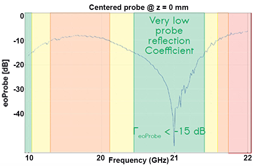
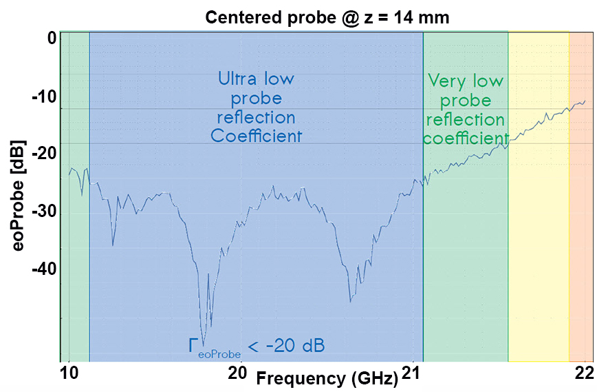
PROBE INTERFERENCE ON HORN ANTENNA
Evaluation from S11
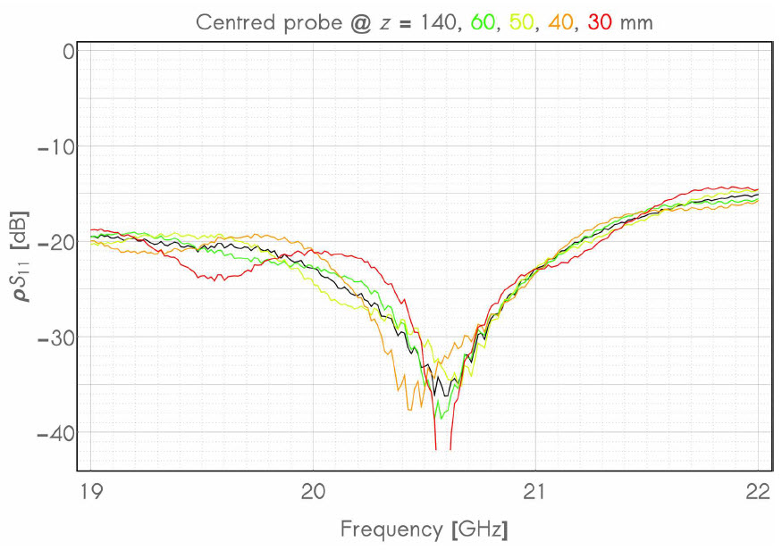
No measurable interference down to 2λ
HYPOTHESES
AT BOUNDARY OF NEAR-FIELD REGION
Negligible effect of probe from ~19 →21 GHz
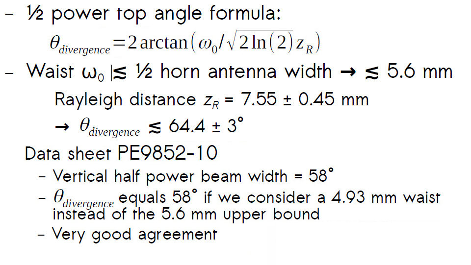
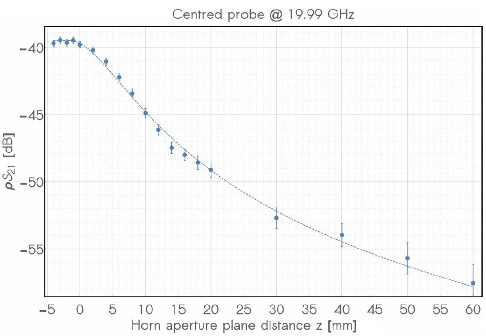
CALCULATION OF BEAM DIVERGENCE
UNCERTAINTY ON S21 VERSUS S21
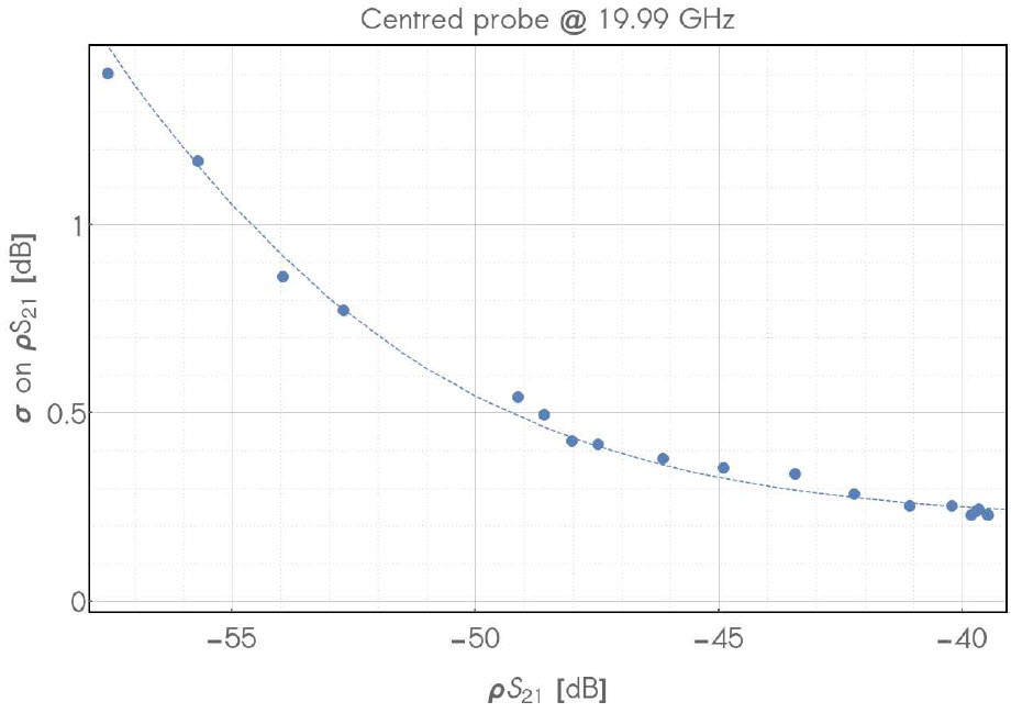
Fit 2 → Scalar Kapteos system calibration noise contributions
● Noise floor
● Asymptotic measurement accuracy (~ 0,2 dB)
RÉSUMÉ OF OBTAINED RESULTS
VNA measurements parameters
– Injected power 0 dBm, → Scalar Kapteos system calibration RBW = 10 Hz, no AVG
● Obtained results (@ 20 GHz & z = 0 mm otherwise written)
– Equiv. optical fibre length → Scalar Kapteos system calibration 7417 ± 35 mm
– Absolute eoSystem dephasing → Scalar Kapteos system calibration 4499 ± 21 rad
– Negligible probe interference for z ≥ λ
– Acceptable probe interference down to z = 0 mm
– Probe effective permittivity ~ 3.6
– RF beam Rayleigh distance → Scalar Kapteos system calibration 7.55 ± 0.45 mm
– Magnitude accuracy on S21: ± 0.23 dB
– Relative phase accuracy on S21: ± 1.7 °
– No de-embedding required
– No incessant calibration required
2D E-FIELD MAPPING
Co-polar 2D mapping (120 points / mapping)
– Spatial step in x direction → Scalar Kapteos system calibration 2 mm
● -11mm ↔ 11 mm (12 values) 11 mm (12 values)
– Spatial step in y direction → Scalar Kapteos system calibration 2 mm
● -9 mm ↔ 11 mm (12 values) 9 mm (10 values)
– Frequential step: 1 GHz
● 19 GHz ↔ 11 mm (12 values) 22 GHz (4 values)
● Graphs
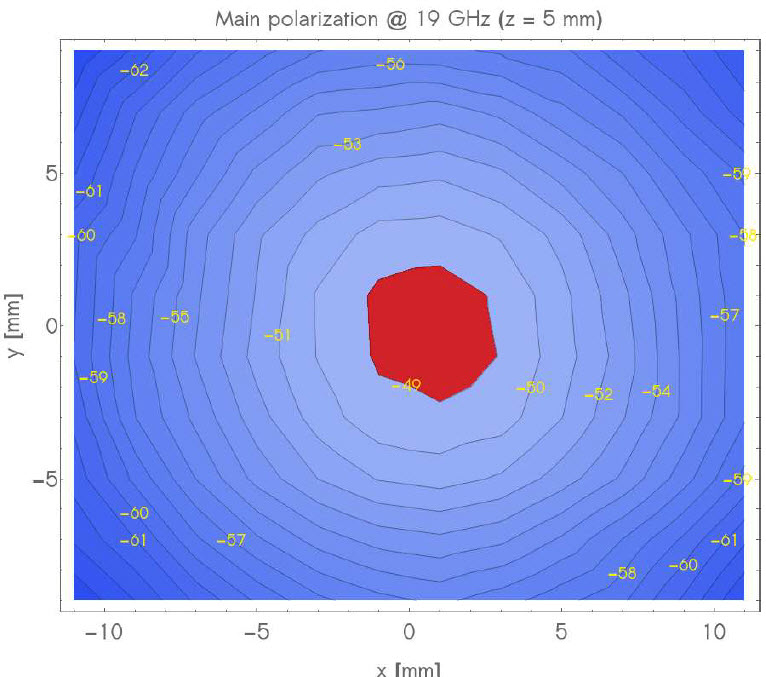
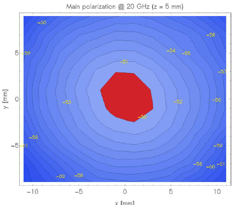
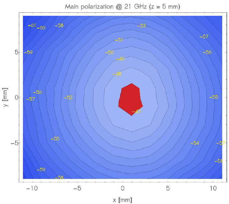
– Modulus – contour lines every 1 dB
● Max in red
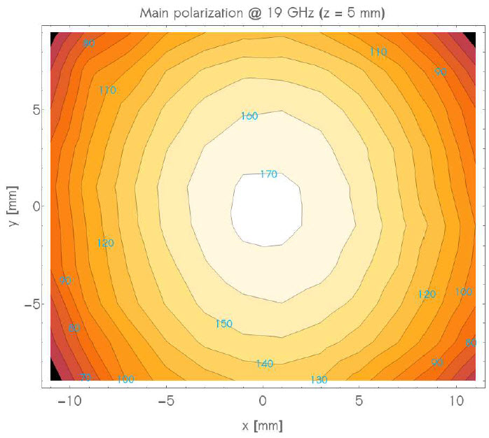
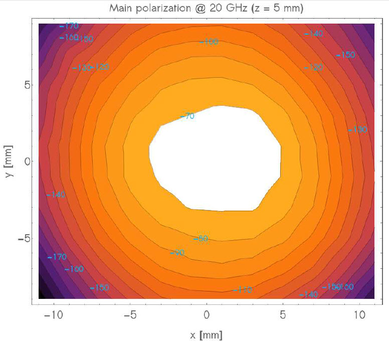
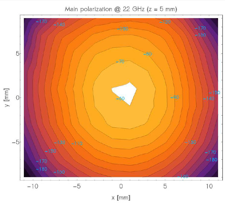
– Phase – contour line every 10°
MAIN POLARISATION
S21 magnitude @ 19 GHz
● S21 phase @ 19 GHz
● S21 magnitude @ 20 GHz
● S21 phase @ 20 GHz
● S21 magnitude @ 21 GHz
● S21 phase @ 22 GHz
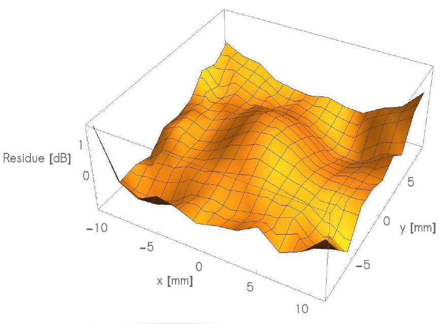
CAUSSIAN BEAM FIT OF MAIN POLARISATION
f = 20 GHz
– Measurement in orange
– Fit in blue
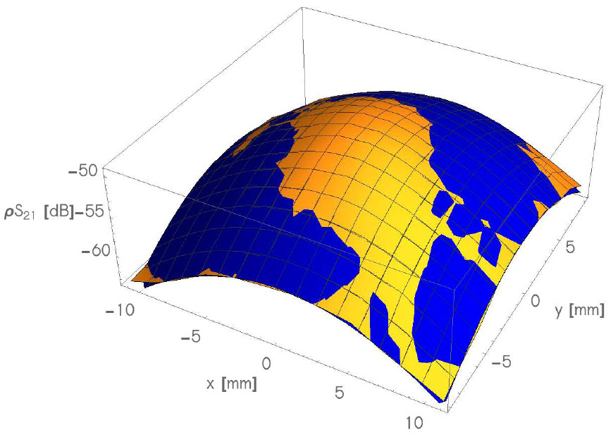
f = 20 GHz
–Residue → RF beam close to a gaussian beam even in the near-field region!
RF BEAM PARAMETERS
Extracted from gaussian fit of 2D field mapping
|
|
f = 19 GHz |
f = 20 GHz |
f = 21 GHz |
f = 22 GHz |
|
Beam |
(0.6 ; -0.1) |
(0.4 ; 0.5) |
(0.8 ; -0.2) |
(0.7 ; 0.0) |
|
Beam waist |
(10.6 ; 10.1) |
(11.7 ; 10.5) |
(10.8 ; 10.9) |
(11.8 ; 11.7) |
|
Max(ρS21) |
-49.1 dB |
-49.9 dB |
-47.9 dB |
-53.4 dB |
● Beam center
– x0 = 0.6 ± 0.2 mm & y0 = 0.1 ± 0.3 mm
● Beam waist @ 1/e² of max power
– ωx = 11.2 ± 0.6 mm & ωy = 10.8 ± 0.7 mm
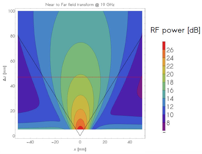
NEAR TO FAR FIELD TRANSFORMATION
● Measurement of magnitude at z = 5 mm
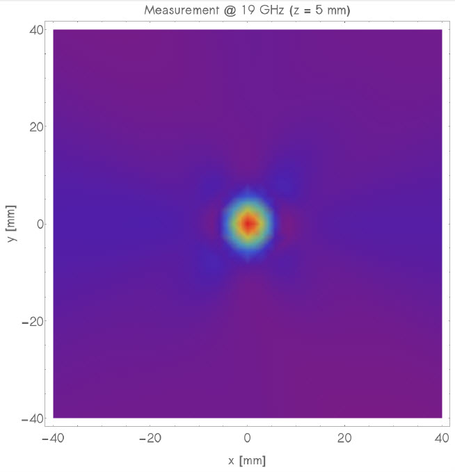
NEAR TO FAR FIELD TRANSFORMATION
● Forward propagation at z = 15
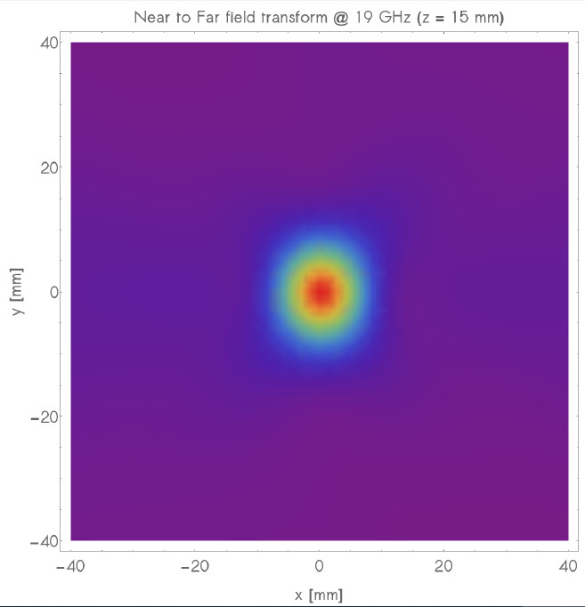
NEAR TO FAR FIELD TRANSFORMATION
● Forward propagation at z = 105 mm
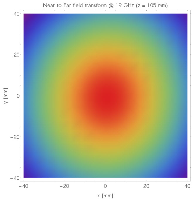
NEAR TO FAR FIELD TRANSFORMATION
● RF power propagation
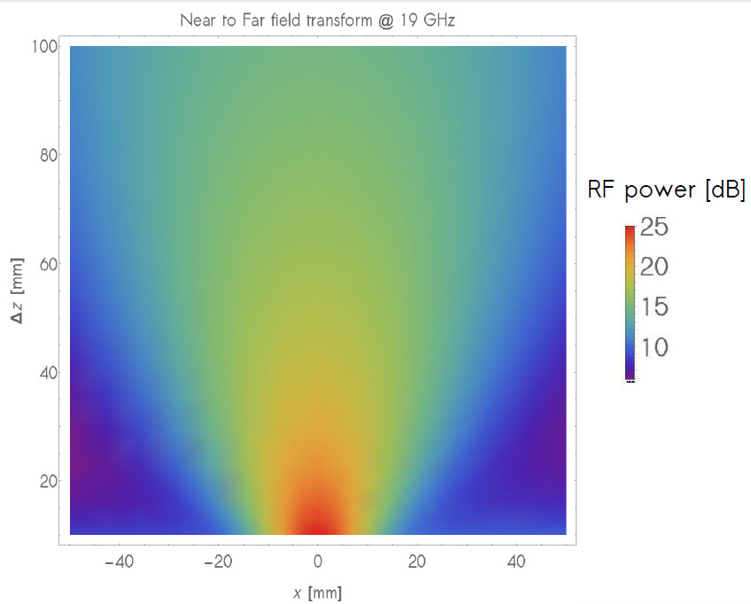
NEAR TO FAR FIELD TRANSFORMATION
● RF phase propagation
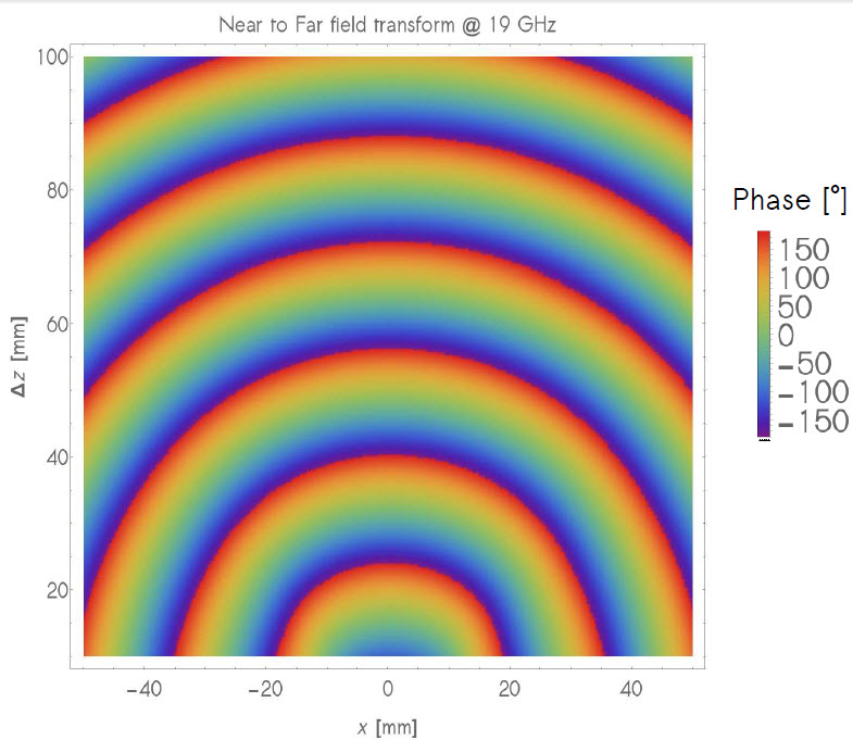
BREACKTHROUGH IN ANTENNA CHARACTERIZATION
● Kapteos technology leads to a comprehensive vectorial near-field characterization of antennas and arrays without any compromise on performances!
![]() Application Note: Vectorial E-field measurement & characterization of Ultra Compact Antennas
Application Note: Vectorial E-field measurement & characterization of Ultra Compact Antennas